Bài thi cuối khóa AIO2024 - Phần 4 (GenAI và LLMs)

DCGAN

Cho kiến trúc mô hình DCGAN đơn giản gồn hai khối Generator, Discriminator được thiết kế như hình vẽ, hãy dựa vào hình để trả lời các câu hỏi liên quan tới phần DCGAN.

import torch
import torch.nn as nn
import torch.nn.functional as F

torch.manual_seed(42)
torch.cuda.manual_seed(42)
torch.backends.cudnn.deterministic = True
torch.backends.cudnn.benchmark = False

class Generator(nn.Module):
    def __init__(self, nz=3):
        super(Generator, self).__init__()
        # Initial input shape: (nz, 1, 1) - assuming input is reshaped to (batch_size, nz, 1, 1)
        self.layer1 = nn.ConvTranspose2d(nz, 1, kernel_size=4, stride=2, padding=1, bias=False)
        self.bn1 = nn.BatchNorm2d(1)
        self.layer2 = nn.ConvTranspose2d(1, 1, kernel_size=4, stride=2, padding=1, bias=False)
        self.bn2 = nn.BatchNorm2d(1)
        self.layer3 = nn.ConvTranspose2d(1, 1, kernel_size=4, stride=2, padding=1, bias=False)
        self.tanh = nn.Tanh()

    def forward(self, x):
        # Input shape: (batch_size, nz, 1, 1)
        x = self.layer1(x)  # Output: (batch_size, 1, 2, 2)
        print(f"Shape after layer1: {x.shape}")
        print(x)
        x = self.bn1(x)
        x = F.relu(x)

        x = self.layer2(x)  # Output: (batch_size, 1, 4, 4)
        print(f"Shape after layer2: {x.shape}")
        x = self.bn2(x)
        x = F.relu(x)

        x = self.layer3(x)  # Output: (batch_size, 1, 8, 8)
        print(f"Shape after layer3: {x.shape}")

        x = self.tanh(x)
        return x

class Discriminator(nn.Module):
    def __init__(self):
        super(Discriminator, self).__init__()
        # Input: (batch_size, 1, 12, 12)
        self.layer1 = nn.Conv2d(1, 1, kernel_size=4, stride=2, padding=1, bias=False)  # 8x8 -> 4x4
        self.layer2 = nn.Conv2d(1, 1, kernel_size=4, stride=2, padding=1, bias=False)  # 4x4 -> 2x2
        self.bn2 = nn.BatchNorm2d(1)

        self.flatten = nn.Flatten()
        self.fc = nn.Linear(2 * 2, 1)
        self.sigmoid = nn.Sigmoid()

    def forward(self, x):
        x = self.layer1(x)
        x = F.leaky_relu(x, 0.2)

        x = self.layer2(x)
        print(f"After layer2: {x}")
        x = self.bn2(x)
        print(f"After bn2: {x}")
        x = F.leaky_relu(x, 0.2)

        x = self.flatten(x)
        x = self.fc(x)
        x = self.sigmoid(x)
        return x

# Initialize models
generator = Generator()
discriminator = Discriminator()

weight_tensor = torch.tensor([[[[ 0.17, -0.22, -0.23,  0.04],
                                [ 0.03, -0.04,  0.21, -0.15],
                                [-0.15, -0.18, -0.04, -0.06],
                                [ 0.15, -0.01,  0.07, -0.10]]],


                              [[[ 0.20,  0.21, -0.22, -0.06],
                                [-0.21,  0.10, -0.21, -0.11],
                                [ 0.24, -0.23,  0.18,  0.02],
                                [ 0.19, -0.12,  0.16,  0.03]]],


                              [[[ 0.01,  0.17, -0.23, -0.20],
                                [ 0.24, -0.15, -0.18, -0.01],
                                [-0.08, -0.03, -0.16,  0.09],
                                [-0.21,  0.02,  0.14,  0.04]]]])
generator.layer1.weight.data = weight_tensor
generator.layer1.weight.data

FNE4DCG01

Sau khi input noise đi qua ConvTranspose2d (layer 1), giá trị output được upscale là?

Lưu ý: Làm tròn tới 4 chữ số thập phân

A. [[ 0.1201, -0.0452], [ 0.0345, 0.0789]]
B. [[-0.0954, 0.1120], [ 0.0543, -0.0876]]
C. [[ 0.0230, 0.45800], [ 0.1100, 0.2350]]
D. [[-0.0303, 0.0054], [-0.1655, -0.0104]]

Đáp án: D

z = torch.tensor([[[[0.52]],
                   [[0.28]],
                   [[0.25]]]])

# Test generator
fake_img = generator(z)

Shape after layer1: torch.Size([1, 1, 2, 2])
tensor([[[[-0.0303,  0.0054],
          [-0.1655, -0.0104]]]], grad_fn=<ConvolutionBackward0>)
Shape after layer2: torch.Size([1, 1, 4, 4])
Shape after layer3: torch.Size([1, 1, 8, 8])

FNE4DCG02

Hãy thực hiện tính toán output của lớp batchnorm tại layer 2 của khối Discriminator sau khi nhận input là fake và real image, đâu là kết quả đúng?

Làm tròn tới 4 chữ số thập phân

A. [[[ 0.5123, -0.8741], [ 1.2094, 0.3567]]], [[[-0.6932, 0.4821], [ 0.1159, -0.9043]]]
B. [[[ 1.0631, 0.7988], [-1.7305, -1.4462]]], [[[ 0.9281, 0.4301], [-0.0217, -0.0217]]]
C. [[[-1.2489, 0.3276], [-0.5421, 1.0873]]], [[[ 0.7654, -0.3198], [ 0.4092, 0.1987]]]
D. [[[ 0.0000, 1.0000], [-1.0000, 0.0000]]], [[[ 0.7071, -0.7071], [ 0.7071, 0.7071]]]

Lưu ý: Làm tròn tới 4 chữ số thập phân

# Test discriminator
img = torch.tensor([[[[0.3100, 0.8400, 0.1900, 0.0900, 0.6100, 0.2200, 0.6400, 0.9200],
          [0.2600, 0.1500, 0.6900, 0.0500, 0.9500, 0.2600, 0.7400, 0.1000],
          [0.1600, 0.5600, 0.6800, 0.8900, 0.9200, 0.4700, 0.4400, 0.5800],
          [0.3800, 0.5200, 0.0300, 0.0900, 0.8400, 0.2100, 0.8900, 0.5500],
          [0.6200, 0.9500, 0.2200, 0.4200, 0.5900, 0.6700, 0.0100, 0.6800],
          [0.2100, 0.5700, 0.8400, 0.4500, 0.4800, 0.4600, 0.9200, 0.7800],
          [0.5800, 0.2000, 0.2300, 0.9000, 0.8600, 0.7900, 0.1100, 0.8900],
          [0.4500, 0.8700, 0.9300, 0.5500, 0.2900, 0.9700, 0.2400, 0.8300]]]])

concatenated_img = torch.cat((img, fake_img), dim=0)
disc_output = discriminator(concatenated_img)

After layer2: tensor([[[[ 0.0203,  0.0127],
          [-0.0594, -0.0513]]],
        [[[ 0.0164,  0.0022],
          [-0.0107, -0.0107]]]], grad_fn=<ConvolutionBackward0>)

After bn2: tensor([[[[ 1.0631,  0.7988],
          [-1.7305, -1.4462]]],
        [[[ 0.9281,  0.4301],
          [-0.0217, -0.0217]]]], grad_fn=<NativeBatchNormBackward0>)

Discriminator output: tensor([[0.6320],
        [0.6101]], grad_fn=<SigmoidBackward0>)

Style Transfer

Cho một kiến trúc đơn giản của bài toán Style Transfer được thiết kế như hình dưới đây:

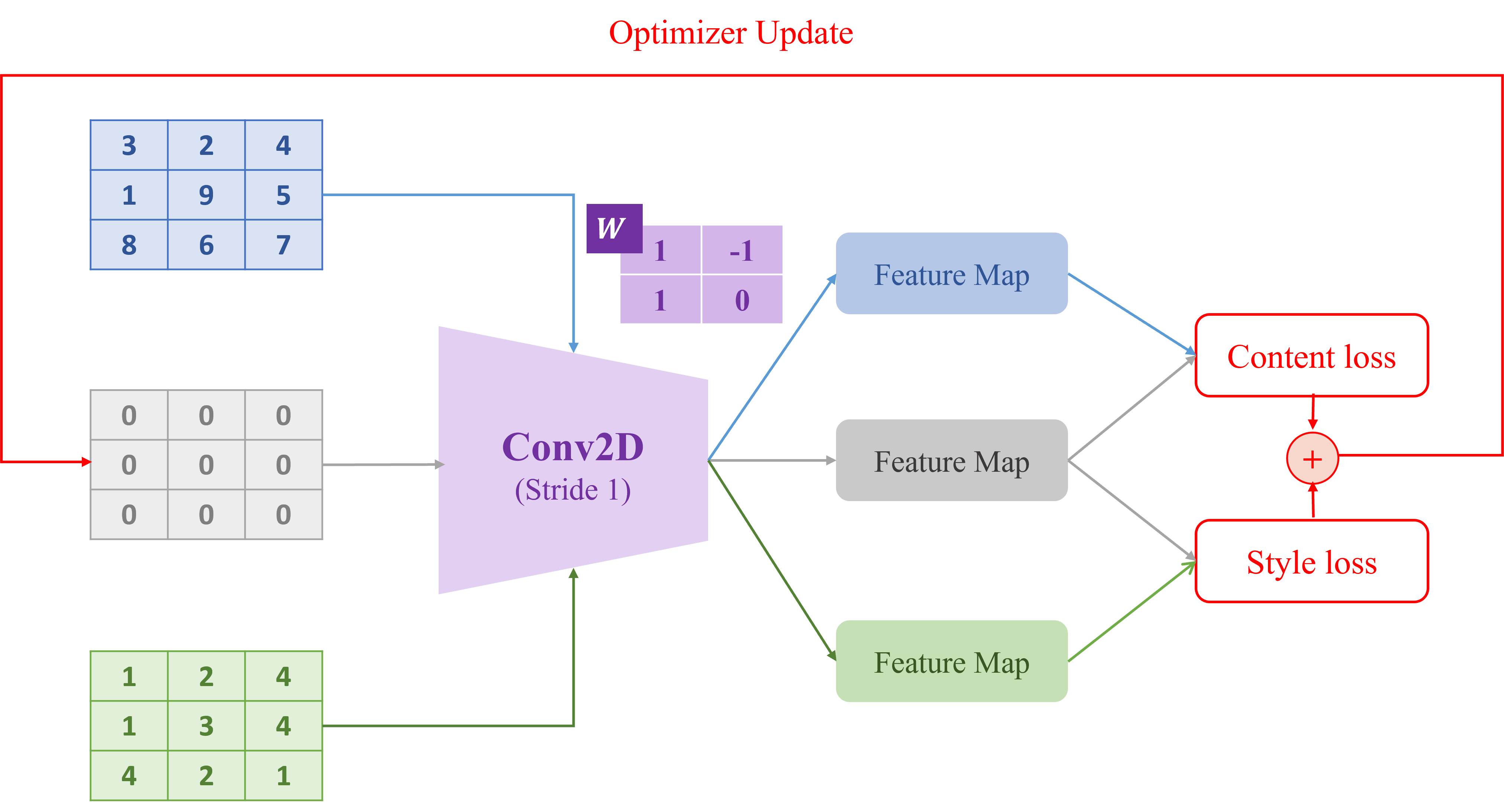
import torch
import torch.nn.functional as F

torch.manual_seed(42)

# INPUTS: 1 channel, 3x3 images (batch size = 1)
content_img = torch.tensor([[[[3.0, 2.0, 4.0],
                              [1.0, 9.0, 5.0],
                              [8.0, 6.0, 7.0]]]], requires_grad=False)

style_img = torch.tensor([[[[1.0, 2.0, 4.0],
                            [1.0, 3.0, 4.0],
                            [4.0, 2.0, 1.0]]]], requires_grad=False)

output_img = torch.zeros_like(content_img, requires_grad=True)

# 1 input channel, 1 output channel, kernel size = 2x2
conv_weight = torch.tensor([[[[1.0, -1.0],
                              [1.0, 0.0]]]], requires_grad=False)  # shape [1, 1, 2, 2]

def simple_cnn(x, weight):
    return F.conv2d(x, weight, stride=1, padding=0)

# Extract feature maps
F_content = simple_cnn(content_img, conv_weight)
F_style = simple_cnn(style_img, conv_weight)
F_output = simple_cnn(output_img, conv_weight)

def gram_matrix(x):
    b, c, h, w = x.shape
    features = x.view(c, h * w)
    return torch.mm(features, features.t())  # shape: [c, c]

def content_loss(F_target, F_content):
    return F.mse_loss(F_target, F_content)

def style_loss(F_target, F_style):
    G_target = gram_matrix(F_target)
    G_style = gram_matrix(F_style)
    return F.mse_loss(G_target, G_style)

FNE4ST01

Hãy tính giá trị của Style Loss (vòng forward đầu tiên) Gợi ý: Tính Style Loss theo phương pháp có trong slide bài style transfer đã được học

A. 36
B. 64
C. 25
D. 49

Đáp án: A

# Tính loss
c_loss = content_loss(F_output, F_content)
s_loss = style_loss(F_output, F_style)
total_loss = c_loss + s_loss

print(f"Content Loss: {c_loss.item():.4f}")
print(f"Style Loss: {s_loss.item():.4f}")
print(f"Total Loss: {total_loss.item():.4f}")

Content Loss: 38.2500
Style Loss: 36.0000
Total Loss: 74.2500

FNE4ST02

Sau bước forward, backward và update đầu tiên (với "learning rate" = 0.01), giá trị của output_image sẽ là gì (làm tròn đến 4 chữ số thập phân)?

A. [[ 0.0200, -0.0150, 0.0400], [ 0.0050, 0.0750, -0.0300], [-0.0100, 0.0600, 0.0100]]
B. [[-0.0050, 0.0350, -0.0250], [ 0.0150, 0.0500, -0.0450], [ 0.0000, 0.0400, -0.0100]]
C. [[ 0.0000, 0.0000, 0.0000], [ 0.0300, 0.0900, -0.0600], [ 0.0050, 0.0550, 0.0050]]
D. [[ 0.0100, 0.0250, -0.0350], [ 0.0100, 0.0850, -0.0500], [ 0.0000, 0.0500, 0.0000]]

Đáp án: D

# Backward
total_loss.backward()

# Learning rate
lr = 0.01
with torch.no_grad():
    output_img -= lr * output_img.grad
    output_img.grad.zero_()

print(output_img.detach()[0,0])

tensor([[ 0.0100,  0.0250, -0.0350],
        [ 0.0100,  0.0850, -0.0500],
        [ 0.0000,  0.0500,  0.0000]])

VAE

import numpy as np
import torch

# Hàm tính z theo Reparameterization Trick
def compute_z(mu, logvar, epsilon):
    sigma = np.exp(0.5 * logvar)
    z = mu + epsilon * sigma
    return sigma, z

# Hàm tính loss
def loss_function(bce_loss, mu, logvar):
    BCE = bce_loss
    KLD = -0.5 * torch.sum(1 + logvar - mu.pow(2) - logvar.exp())
    return BCE + KLD

mu_np = np.array([2.13, -0.94])
logvar_np = np.array([-4.72, -4.27])
epsilon_np = np.array([-1.05, -0.05])

FNE4VAE01

Mô tả: Mô hình VAE Encoder trong ảnh nhận đầu vào là hình ảnh (minh họa) và đầu ra gồm mean ( $\mu$ ) và log(variance) ( $logvar$ ) có giá trị được cho trước như trong hình. Ngoài ra, trong Reparameterization Trick, cho trước giá trị của $\epsilon$ như trong hình.

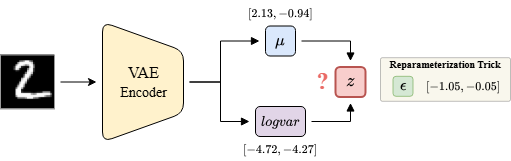
Câu hỏi: Hãy tính các giá trị của $z$ và chọn đáp án có kết quả gần đúng nhất.

A. $[2.39, 1.82]$
B. $[1.39, 2.29]$
C. $[2.03, -0.94]$
D. $[-1.27, -0.82]$

Đáp án: C

# Tính sigma và z
sigma, z = compute_z(mu_np, logvar_np, epsilon_np)
print(f"Sigma: {sigma}")

Sigma: [2.03085877 -0.94591223]

FNE4VAE02

Mô tả: Sau khi thu được vector tiềm ẩn $z$ , ta truyền $z$ qua Decoder của mô hình VAE để tái tạo lại hình ảnh đầu vào. Giả sử mô hình đã được huấn luyện tốt và các thành phần $log(var)$ và $\epsilon$ trong công thức Reparameterization Trick không gây ảnh hưởng quá lớn. Cụ thể giá trị của $\epsilon$ (hoặc tác động của nó) không làm cho $z$ bị lệch quá xa so với $\mu$ , đặc biệt trong trường hợp độ lệch chuẩn $\sigma$ nhỏ. Khi đó, nếu $\sigma \cdot \epsilon$ nhỏ thì:

z = \mu + \sigma \cdot \epsilon \approx \mu

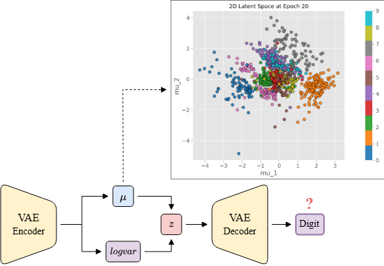
Ta dựa vào $\mu$ để vẽ không gian tiềm ẩn (latent space) 2 chiều gồm $\mu_1$ và $\mu_2$ như hình vẽ, với các điểm tròn có màu sắc tương ứng với nhãn là một con số từ 0-9. Ví dụ: các điểm tròn màu xanh biển đậm là số 0, điểm tròn màu cam là số 1, ...

Câu hỏi: Với $z$ vừa tính được ở câu trước, đầu ra của VAE Decoder là số?

A. số 2
B. số 0
C. số 7
D. số 1

Đáp án: D

Nhìn vào hình vẽ, ta thấy rằng điểm $z$ nằm gần các điểm tròn màu cam (số 1) hơn so với các điểm tròn khác. Do đó, đầu ra của VAE Decoder sẽ là số 1.

FNE4VAE03

Câu hỏi: Tiếp tục với model trên, giả sử BCE loss = 0.1. Tính loss tổng của model VAE đã cho?

A. 7.61
B. 7.11
C. 6.21
D. 6.31

Đáp án: D

mu = torch.tensor(mu_np, dtype=torch.float32)
logvar = torch.tensor(logvar_np, dtype=torch.float32)

bce_loss = torch.tensor(0.1)

total_loss = loss_function(bce_loss, mu, logvar)

print(f"Total Loss: {total_loss.item():.2f}")

Total Loss: 6.3166985511779785

Diffusion

import torch
import random
import os
import torch.nn as nn
import torch.nn.functional as F
import torch.optim as optim
from torch.utils.data import DataLoader
from torchvision import datasets, transforms
import matplotlib.pyplot as plt
import numpy as np
from tqdm import tqdm

seed = 43
random.seed(seed)
os.environ['PYTHONHASHSEED'] = str(seed)
np.random.seed(seed)
torch.manual_seed(seed)
torch.cuda.manual_seed(seed)
torch.cuda.manual_seed_all(seed)
torch.backends.cudnn.deterministic = True
torch.backends.cudnn.benchmark = False

device = torch.device("cuda")

diffusion_steps = 10
beta_start = 0.01
beta_end = 0.1

def round_tensor(tensor):
    return torch.round(tensor, decimals=3)

def format_tensor(tensor):
    if isinstance(tensor, torch.Tensor):
        if tensor.ndim == 0 or tensor.numel() == 1:
            return f"{tensor.item():.3f}"
        else:
            return "[" + ", ".join(f"{v:.3f}" for v in tensor.tolist()) + "]"
    elif isinstance(tensor, (float, int)):
        return f"{tensor:.3f}"
    else:
        return str(tensor)

class DiffusionModel:
    def __init__(self, num_steps=diffusion_steps, beta_start=beta_start, beta_end=beta_end):
        self.num_steps = num_steps
        self.betas = torch.linspace(beta_start, beta_end, num_steps)
        self.alphas = 1 - self.betas
        self.alphas_cumprod = torch.cumprod(self.alphas, dim=0)
        self.sqrt_alphas_cumprod = torch.sqrt(self.alphas_cumprod)
        self.sqrt_one_minus_alphas_cumprod = torch.sqrt(1 - self.alphas_cumprod)
        self.one_val = torch.tensor(1.0)
        self.prng_generator = torch.Generator()

    def forward_diffusion(self, x0, t):
        noise = round_tensor(torch.Tensor([-0.55, -0.62]))

        sqrt_alpha_cumprod_t = round_tensor(self.sqrt_alphas_cumprod[t].view(-1, 1))
        sqrt_one_minus_alpha_cumprod_t = round_tensor(self.sqrt_one_minus_alphas_cumprod[t].view(-1, 1))
        noisy_x = round_tensor(sqrt_alpha_cumprod_t * x0 + sqrt_one_minus_alpha_cumprod_t * noise)

        print(f"{'x0:':<40}{format_tensor(x0)}")
        print(f"{'noise:':<40}{format_tensor(noise)}")
        print(f"{'sqrt_alphas_cumprod[t]:':<40}{format_tensor(sqrt_alpha_cumprod_t)}")
        print(f"{'sqrt_one_minus_alphas_cumprod[t]:':<40}{format_tensor(sqrt_one_minus_alpha_cumprod_t)}")
        print(f"{'noisy_x:':<40}{noisy_x}")

    def _get_previous_timestep(self, timestep):
        return timestep - 1 if timestep > 0 else -1

    def _calculate_variance(self, timestep):
        return self.betas[timestep]

    def reverse_diffusion(self, current_timestep, current_latents, noise_prediction):
        previous_timestep = self._get_previous_timestep(current_timestep)
        previous_timestep = (torch.tensor(previous_timestep)).long().item()

        cumprod_alpha_current = round_tensor(self.alphas_cumprod[current_timestep])
        cumprod_alpha_previous = round_tensor(self.alphas_cumprod[previous_timestep]) if previous_timestep >= 0 else self.one_val

        cumprod_beta_current = round_tensor(1 - cumprod_alpha_current)
        cumprod_beta_previous = round_tensor(1 - cumprod_alpha_previous)

        current_alpha_ratio = round_tensor(cumprod_alpha_current / cumprod_alpha_previous)
        current_beta_ratio = round_tensor(1 - current_alpha_ratio)

        predicted_x0 = round_tensor((current_latents - cumprod_beta_current.sqrt() * noise_prediction) / cumprod_alpha_current.sqrt())

        original_coefficient = round_tensor((cumprod_alpha_previous.sqrt() * current_beta_ratio) / cumprod_beta_current)
        latent_coefficient = round_tensor(current_alpha_ratio.sqrt() * cumprod_beta_previous / cumprod_beta_current)

        prior_mean_prediction = round_tensor(original_coefficient * predicted_x0 + latent_coefficient * current_latents)

        variance_term = 0
        if current_timestep > 0:
            target_device = noise_prediction.device
            noise_component = round_tensor(torch.Tensor([-0.55, -0.62]))
            variance_term = round_tensor(self._calculate_variance(current_timestep).sqrt() * noise_component)

        prior_sample_prediction = round_tensor(prior_mean_prediction + variance_term)

        print(f"{'current_timestep:':<40}{(current_timestep)}")
        print(f"{'previous_timestep:':<40}{(previous_timestep)}")
        print(f"{'cumprod_alpha_current:':<40}{format_tensor(cumprod_alpha_current)}")
        print(f"{'cumprod_alpha_previous:':<40}{format_tensor(cumprod_alpha_previous)}")
        print(f"{'cumprod_beta_current:':<40}{format_tensor(cumprod_beta_current)}")
        print(f"{'cumprod_beta_previous:':<40}{format_tensor(cumprod_beta_previous)}")
        print(f"{'current_alpha_ratio:':<40}{format_tensor(current_alpha_ratio)}")
        print(f"{'current_beta_ratio:':<40}{format_tensor(current_beta_ratio)}")
        print(f"{'predicted_x0:':<40}{format_tensor(predicted_x0)}")
        print(f"{'original_coefficient:':<40}{format_tensor(original_coefficient)}")
        print(f"{'latent_coefficient:':<40}{format_tensor(latent_coefficient)}")
        print(f"{'--> prior_mean_prediction:':<40}{format_tensor(prior_mean_prediction)}")
        print(f"{'variance_term:':<40}{format_tensor(variance_term)}")
        print(f"{'prior_sample_prediction:':<40}{format_tensor(prior_sample_prediction)}")

noise_scheduler = DiffusionModel()

FNE4DF01

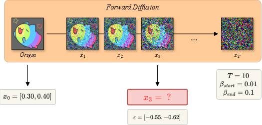
Mô tả: Hình bên minh hoạ quá trình thêm nhiễu vào hình ảnh qua từng bước (step) $t$ trong các mô hình Diffusion. Bắt đầu từ $x_0$ (Origin), thêm nhiễu qua từng bước, tối đa $T=10$ bước với mức độ nhiễu từ $\beta_{start}=0.01$ đến $\beta_{end}=0.1$ ( biết $\beta = [\beta_1, \beta_2, \ldots, \beta_{10}]$ ). Ví dụ cụ thể, tại bước đầu tiên, mô hình sẽ nhận đầu vào là Origin và trả về ảnh đã thêm nhiễu $x_1$ , và lặp lại như thế cho các step tiếp theo $t=t+1$ cho tới khi nhận được ảnh nhiễu hoàn toàn (pure noise) $x_T$ . Ngoài ra, luôn cố định $\epsilon$ khi tính Parameterization Trick bằng các giá trị như trong hình.

Yêu cầu:

Làm tròn tất cả giá trị tính toán đến 3 chữ số thập phân cho mỗi bước tính.
Hãy tính $x_3$ và chọn đáp án đúng gần nhất.

Trắc nghiệm:

A. $[0.137, 0.217]$
B. $[0.157, 0.237]$
C. $[0.177, 0.257]$
D. $[0.197, 0.277]$

Đáp án: B

x_0 = torch.Tensor([0.300, 0.400])
noise_scheduler.forward_diffusion(x_0, 2)
# 2 là index trong code, với giả thuyết thì tương ứng vị trí thứ 3

x0:                                     [0.300, 0.400]
noise:                                  [-0.550, -0.620]
sqrt_alphas_cumprod[t]:                 0.970
sqrt_one_minus_alphas_cumprod[t]:       0.243
noisy_x:                                tensor([[0.1570, 0.2370]])

FNE4DF02

Mô tả: Hình bên mô tả quá trình khử nhiễu qua từng bước (step) $t$ sau khi đã làm nhiễu ảnh đầu vào thành nhiễu hoàn toàn (pure noise) sau $T$ bước trước đó. Cụ thể hơn, mô hình sẽ khử nhiễu một cách tuần tự theo từng step, nghĩa là đầu tiên mô hình nhận pure noise làm đầu vào và trả về $x_9$ đã giảm bớt nhiễu, sau đó, tiếp tục nhận $x_9$ làm đầu vào và trả về $x_8$ , tương tự như thế cho tới khi nhận được ảnh $x_0$ (generation).

Cho trước các siêu tham số sau:

$T=10$ bước.
Mức độ nhiễu từ $\beta_{start}=0.01$ đến $\beta_{end}=0.1$ . (biết $\beta = [\beta_1, \beta_2, \ldots, \beta_{10}]$ )
Ảnh đã thêm nhiễu $x_8$ .
$\epsilon_{\theta}$ là nhiễu được mô hình dự đoán khi nhận đầu vào là $x_8$ .
Luôn cố định $\epsilon$ khi dùng Parameterization Trick với giá trị như trong hình.

Yêu cầu:

Làm tròn tất cả giá trị tính toán đến 3 chữ số thập phân cho mỗi bước tính.
Hãy tính $x_7$ và chọn đáp án đúng gần nhất.

Trắc nghiệm:

A. $[-0.357, -0.443]$
B. $[-0.387, -0.473]$
C. $[-0.417, -0.503]$
D. $[-0.447, -0.533]$

Đáp án: A

noise_scheduler.reverse_diffusion(current_timestep=7,
                                  current_latents=torch.Tensor([-0.15, -0.20]),
                                  noise_prediction=torch.Tensor([0.30, 0.40]))
# current_timestep=7 là index trong code, với giả thuyết thì tương ứng vị trí thứ 8

current_timestep:                       7
previous_timestep:                      6
cumprod_alpha_current:                  0.690
cumprod_alpha_previous:                 0.750
cumprod_beta_current:                   0.310
cumprod_beta_previous:                  0.250
current_alpha_ratio:                    0.920
current_beta_ratio:                     0.080
predicted_x0:                           [-0.382, -0.509]
original_coefficient:                   0.223
latent_coefficient:                     0.774
--> prior_mean_prediction:              [-0.201, -0.268]
variance_term:                          [-0.156, -0.175]
prior_sample_prediction:                [-0.357, -0.443]

Flow Matching

import torch
import torch.nn as nn

class Flow(nn.Module):
    def __init__(self) -> None:
        super().__init__()

        self.linear = nn.Linear(2, 1)

        with torch.no_grad():
            self.linear.weight.copy_(torch.tensor([[0.3, 0.8]]))
            self.linear.bias.copy_(torch.tensor([0]))

            self.linear.weight.requires_grad = False
            self.linear.bias.requires_grad = False

    def forward(self,  t: torch.Tensor, x: torch.Tensor) -> torch.Tensor:
        t = t.unsqueeze(0).float()
        x = torch.cat([x, t], dim=0)
        x = self.linear(x)
        x = nn.Tanh()(x)
        return x

# Khởi tạo model - loss
model = Flow()
loss_fn = nn.MSELoss()

# Giá trị cho trước
x_1 = torch.tensor([0.6])
x_0 = torch.tensor([-0.2])
t = torch.tensor(0.6)

FNE4FM01

Cho kiến trúc Flow Matching được thiết kế đơn giản như hình trên.

Biết rằng $x_0$ = -0.2, $x_1$ = 0.6, t = 0.6 và model (linear không có bias).

Câu hỏi: Hãy tính loss của mạng trên (kết quả cuối cùng được làm tròn đến chữ số thập phân thứ 2)

A. 0.08
B. 0.11
C. 0.14
D. 0.17

Đáp án: A

x_t = (1 - t) * x_0 + t*x_1
pred = model(t, x_t)
target = x_1 - x_0

loss = loss_fn(pred, target)
print("loss:  ", loss.item())

loss:   0.08355613052845001

FNE4FM02

Cho sampling process của Flow Matching như hình trên.

Biết rằng $x_{0.1}$ = 0.7 (step 1), số step n=10 và model (linear không có bias) như trong hình 2.

Câu hỏi: Hãy tính $x_{0.3}$ (step 3).

A. 0.8111
B. 0.8131
C. 0.8144
D. 0.8234

Đáp án: B

class Flow2(nn.Module):
    def __init__(self) -> None:
        super().__init__()

        self.linear = nn.Linear(2, 1)

        with torch.no_grad():
            self.linear.weight.copy_(torch.tensor([[0.7, 0.9]]))
            self.linear.bias.copy_(torch.tensor([0]))

            self.linear.weight.requires_grad = False
            self.linear.bias.requires_grad = False

    def forward(self,  t: torch.Tensor, x: torch.Tensor) -> torch.Tensor:
        t = t.unsqueeze(0).float()
        x = torch.cat([x, t], dim=0)
        x = self.linear(x)
        x = nn.Tanh()(x)
        return x

# Khởi tạo model
model = Flow2()

# Các giá trị cho trước
x1 = torch.tensor([0.7])
steps = 10

delta = 1/steps
t1 = torch.tensor(0) + delta

# Tính toán x2
x2 = x1 + delta * model(t1, x1)
t2 = t1 + delta

# Tính toán x3
x3 = x2 + delta * model(t2, x2)
print("x3:  ", x3.item())

x3:   0.8131197094917297

PretrainingGPT

Xây dựng bộ tách từ và mô hình cho bước tiền huấn luyện dựa trên kiến trúc của mô hình GPT2

Thay thế code vào các đoạn "None" tương tự mẫu bên dưới để trả lời các câu hỏi.
Không được thay đổi code ở các đoạn ngoài vùng yêu cầu.

# START YOUR CODE
a = None
b = None
# END YOUR CODE

LINK CODE

Lưu ý:

Chạy code hoàn chỉnh để trả lời cho cả 3 câu FNE4PGPT01, FNE4PGPT02, FNE4PGPT03.
Lưu model lên hugging face để chạy code cho phần bài tập PEFT

FNE4PGPT01

Bộ từ điển sau khi huấn luyện dựa vào mô tả trong phần code có kích thước là bao nhiêu?

A. 50257
B. 46744
C. 38156
D. 27057

Đáp án: B

trainer = BpeTrainer(
    vocab_size=50257,
    min_frequency=50,
    special_tokens=["<pad>", "<unk>", "<s>"]
)

Length Vocab: 46744

FNE4PGPT02

Mô hình GPT2 sau khi khởi tạo dựa vào mô tả trong phần code có số lượng tham số xấp xỉ với?

A. 200 triệu tham số
B. 250 triệu tham số
C. 300 triệu tham số
D. 350 triệu tham số

Đáp án: D

config = GPT2Config(
    vocab_size=tokenizer.vocab_size,
    n_positions=1024,
    n_ctx=1024,
    n_embd=1024,
    n_layer=24,
    n_head=16,
    bos_token_id=tokenizer.bos_token_id
)

Tổng số tham số: 351,225,856
Tham số huấn luyện được: 351,225,856

FNE4PGPT03

Truyền đoạn văn bản sau: "I am delving into ancient history to write my thesis" vào đoạn code trong phần hướng dẫn cho hàm "inference" thì kết quả trả về của "logits.shape[1]" là bao nhiêu?

A. 10
B. 11
C. 12
D. 13

Đáp án: B

outputs = model(**inputs)

Logits Shape: 11

PEFT

Sử dụng mô hình GPT2 đã khởi tạo từ phần Pre-Training để tiếp tục áp dựng các phương pháp tối ưu cho quá trình Fine-Tuning

Thay thế code vào các đoạn "None" tương tự mẫu bên dưới để trả lời các câu hỏi.
Không được thay đổi code ở các đoạn ngoài vùng yêu cầu.

# START YOUR CODE
a = None
b = None
# END YOUR CODE

LINK CODE

FNE4PEFT01

Phần trăm các tham số cần huấn luyện cho mô hình GPT2 sau khi áp dụng phương pháp Prefix-Tuning và Prompt-Tuning lần lượt xấp xỉ với?

A. 0.279 và 0.006
B. 0.006 và 0.279
C. 0.179 và 0.06
D. 0.06 và 0.179

Đáp án: A

peft_config = PrefixTuningConfig(
    task_type=TaskType.CAUSAL_LM,
    num_virtual_tokens=20
)

peft_config = PromptTuningConfig(
    task_type=TaskType.CAUSAL_LM,
    num_virtual_tokens=20
)

trainable params: 983,040 || all params: 352,208,896 || trainable%: 0.2791
trainable params: 20,480 || all params: 351,246,336 || trainable%: 0.0058

FNE4PEFT02

Mô hình GPT2 sau khi khởi tạo dựa vào mô tả trong phần code có thể áp dụng phương pháp LoRA cho những layers nào?

A. c_query, c_value, c_key
B. c_attn, c_proj, c_fc
C. q_proj, k_proj, v_proj, o_proj
D. gate_proj, up_proj, down_proj

Đáp án: B

Hãy xem xét cấu trúc của một khối Transformer trong GPT-2. Nó chủ yếu bao gồm hai phần chính: cơ chế tự chú ý (self-attention) và mạng truyền thẳng (feed-forward network). Đọc về danh sách các layer ở đây: Link

"c_attn" (Convolutional Attention): Đây là lớp "Conv1D" trong thư viện "transformers" của Hugging Face, được sử dụng để tạo ra các vector query, key, và value trong cơ chế tự chú ý (self-attention).
"c_proj" (Convolutional Projection): Đây là lớp "Conv1D" theo sau cơ chế tự chú ý, có nhiệm vụ chiếu (project) output của các đầu chú ý (attention heads) trở lại không gian ban đầu của embedding.
"c_fc" (Convolutional Fully Connected): Đây là lớp "Conv1D" đầu tiên trong mạng truyền thẳng (feed-forward network) của khối Transformer, có vai trò mở rộng chiều dữ liệu.

Trong khi đó, các lựa chọn khác không phù hợp với kiến trúc của GPT-2 trong thư viện "transformers":

A. c_query, c_value, c_key: Các thành phần này không tồn tại dưới dạng các lớp riêng lẻ trong triển khai GPT-2 của Hugging Face. Thay vào đó, chúng được tính toán gộp bên trong lớp "c_attn".
C. q_proj, k_proj, v_proj, o_proj: Tên các lớp này (query, key, value, output projection) là quy ước đặt tên phổ biến trong các kiến trúc Transformer khác như Gemma hoặc LLaMA, nhưng không phải trong GPT-2.
D. gate_proj, up_proj, down_proj: Đây là các tên lớp thường thấy trong các kiến trúc mô hình ngôn ngữ lớn khác như LLaMA, không phải GPT-2.

FNE4PEFT03

Phần trăm số lượng các tham số sau khi áp dụng LoRA dựa vào các cài đặt tham số trong code là?

A. 0.12
B. 0.22
C. 0.32
D. 0.42

Đáp án: B

lora_config = LoraConfig(
    task_type=TaskType.CAUSAL_LM,
    r=8,
    lora_alpha=16,
    lora_dropout=0.05,
    target_modules=["c_attn"]
)

trainable params: 786,432 || all params: 352,012,288 || trainable%: 0.2234

Prompting and Reasoning

Bài tập thực hành xây dựng một mô hình ngôn ngữ lớn có khả năng làm toán thông qua tích hợp cú pháp suy luận.

Chúng ta sẽ huấn luyện mô hình với LoRA trên tập dataset GSM8K bằng thư viện "unsloth" và "trl".

Để hoàn thành bài tập này, bạn cần:

Điền code của bạn vào các dấu "..." (minh hoạ bên dưới)
KHÔNG được thay đổi code ở các đoạn ngoại trừ vùng được đánh dấu như sau:

## TODO: Complete the following code by replacing ... with your code
a = ... # Fill your code here
# or
... # Fill your code here, also
# or even
... = "abc" # Fill your code here, too
## END

Link bài thực hành code: Colab

LƯU Ý: File colab trên chạy cho 3 câu hỏi đầu tiên dưới đây.

FNE4MCQA01

Số lượng sample sau khi trích xuất answer của tập GSM8K là bao nhiêu:

A. 7471
B. 7473
C. 7475
D. 7477

Đáp án: B

Dataset({
    features: ['question', 'answer', 'reasoning', 'prompt'],
    num_rows: 7473
})

FNE4MCQA02

Số lượng trainable parameters (tham số có thể cập nhật đạo hàm trong quá trình huấn luyện) là bao nhiêu:

A. 4,587,520
B. 3,192,860
C. 5,934,024
D. 3,549,250

Đáp án: A

base_model, tokenizer = FastLanguageModel.from_pretrained(
    model_name=MODEL_NAME_OR_PATH,
    max_seq_length=MAX_SEQ_LEN,
    load_in_4bit=False,
    fast_inference=True,
    max_lora_rank=8,
    gpu_memory_utilization=0.9,
)

training_args = GRPOConfig(
    learning_rate=3e-5,
    optim="paged_adamw_8bit",
    per_device_train_batch_size=2,
    gradient_accumulation_steps=4,
    max_grad_norm=1,
    num_train_epochs=1,
    logging_first_step=True,
    max_steps=-1,
    save_steps=20,
    logging_steps=10,
    warmup_ratio=0.1,
    num_generations=2,
    max_prompt_length=max_prompt_length,
    max_completion_length=MAX_SEQ_LEN - max_prompt_length,
    report_to="none",
    output_dir="gsm8k_reasoning",
)

grpo_trainer = GRPOTrainer(
    model=model,
    train_dataset=train_dataset,
    processing_class=tokenizer,
    args=training_args,
    reward_funcs=[match_format_exactly, match_format_approximately, check_answer, check_numbers],
)

==((====))==  Unsloth - 2x faster free finetuning | Num GPUs used = 1
   \\   /|    Num examples = 7,473 | Num Epochs = 1 | Total steps = 1,868
O^O/ \_/ \    Batch size per device = 2 | Gradient accumulation steps = 4
\        /    Data Parallel GPUs = 1 | Total batch size (2 x 4 x 1) = 8
 "-____-"     Trainable parameters = 4,587,520/3,217,337,344 (0.14% trained)
Unsloth: Will smartly offload gradients to save VRAM!

FNE4MCQA03

Giá trị của reward sau khi huấn luyện mô hình ở training step đầu tiên là bao nhiêu?

A. 0.354892
B. 1.136745
C. 1.562500
D. -0.875000

Đáp án: C

[ 5/1868 01:53 < 19:36:03, 0.03 it/s, Epoch 0.00/1]

Step	Training Loss	reward	reward_std	completion_length	kl	rewards / match_format_exactly	rewards / match_format_approximately	rewards / check_answer	rewards / check_numbers
1	-0.000000	1.562500	1.325825	264.375000	0.000000	0.750000	0.312500	0.187500	0.312500

FNE4MCQA04

Đâu là kĩ thuật prompting không làm tăng hiệu suất của LLM như các kĩ thuật còn lại:

A. Zero-shot CoT Prompting
B. Tree-of-Thought Prompting
C. Chain-of-Thought Prompting
D. Zero-shot Prompting

Đáp án: D

Zero-shot Prompting này hoàn toàn dựa vào kiến thức đã được huấn luyện trước đó của mô hình. Nó không chủ động hướng dẫn mô hình cách suy luận hay chia nhỏ vấn đề. Vì vậy, nó được coi là phương pháp nền tảng (baseline) và thường có hiệu suất thấp hơn trong các tác vụ phức tạp so với các kỹ thuật khác.

RAG

Bài tập thực hành xây dựng một hệ thống retrieval augmented generation (RAG) với thư viện "LangChain".

Chúng ta sẽ xây dựng RAG pipeline để mô hình LLM có thể hỏi đáp về chủ đề Parameter-Efficient Fine-Tuning (PEFT) thông qua các paper đã được tải về ở local drive.

Để hoàn thành bài tập này, bạn cần:

Điền code của bạn vào các dấu "..." (minh hoạ bên dưới)
KHÔNG được thay đổi code ở các đoạn ngoại trừ vùng được đánh dấu như sau:

## TODO: Complete the following code by replacing ... with your code
a = ... # Fill your code here
# or
... # Fill your code here, also
# or even
... = "abc" # Fill your code here, too
## END

Link bài thực hành code: Colab.

LƯU Ý: File colab trên chạy cho cả 3 câu hỏi dưới đây.

FNE4RAG01

Có bao nhiêu text chunks được chia ra khi sử dụng "RecursiveCharacterTextSplitter" được khai báo bằng các tham số như yêu cầu đề bài:

A. 974
B. 971
C. 975
D. 973

Đáp án: A

text_splitter = RecursiveCharacterTextSplitter(
    separators=["\n\n", "\n", " ", ""],
    chunk_size=1024,
    chunk_overlap=128,
)

Split all pdf documents into 974 text chunks.

FNE4RAG02

Sử dụng retriever đã xây, văn bản đầu tiên khi tìm kiếm với cụm từ "background and mathematics of low-rank adaptation" bắt đầu bằng cụm từ nào dưới đây?

A. The improvements of LoRA are mimicked in two streams: (1) Adaptability [6,12,2]: This refers to the celerity with which the method converges to an optimal or near-optimal state.
B. the weight update Wcan be approximated by the product of two lower-rank matrices, BAW. Evidently, this specific factorization is not necessarily the optimal low-rank approximation of the original W. ...
C. overhead. LoRA constructs this low-rank adaptation matrix through an intuitive design, positing that ...
D. have demonstrated its usefulness in various adaptation tasks. The proposed HRA method bridges the gap between low-rank and orthogonal adaptation strategies. It simplifies the implementation of OFT while inheriting its theoretical guarantees on the retention of pre-training knowledge. ... \

Đáp án: C

results = retriever.invoke("background and mathematics of low-rank adaptation")

overhead. LoRA constructs this low-rank adaptation matrix through an intuitive design, positing that
the weight update Wcan be approximated by the product of two lower-rank matrices, BAW.
Evidently, this specific factorization is not necessarily the optimal low-rank approximation of the
original W.
The improvements of LoRA are mimicked in two streams: (1) Adaptability [6,12,2]: This refers to
the celerity with which the method converges to an optimal or near-optimal state. The approximation
Preprint. Under review.arXiv:2409.15371v9  [cs.CL]  16 May 2025

FNE4RAG03

Khi chạy RAG chain với câu hỏi: "What is the mathematical background of low-rank adaptation?", chúng ta nhận được câu trả lời (gần đúng nhất) nào dưới đây (field "answer"):

LƯU Ý: chạy nhiều lần và chọn câu trả lời có số lần xuất hiện nhiều nhất. Chọn đáp án nào mà có số chữ sai lệch ít nhất.

A. Low-rank adaptation approximates the weight update by using the product of two lower-rank matrices.
B. Several studies have aimed to improve LoRA's performance, such as Laplace-LoRA, LoRA Dropout, LoRA+, and MoSLoRA.
C. LoRA adds trainable pairs of rank decomposition matrices in parallel to existing weight matrices.
D. LoRA in PEFT can be combined with prex-embedding tuning (LoRA+PE) or prex-layer tuning (LoRA+PL) by inserting special tokens and treating their embeddings as trainable parameters.

Đáp án: A

llm = ChatGoogleGenerativeAI(
    model="gemini-2.0-flash",
    temperature=0.0,
    top_k=1,
    google_api_key="AIzaSyA6XCTHoku7uUsQs_tpcKIKjkuUeDYabhQ",
    max_retries=2,
    timeout=30,
    max_tokens=1024,
)

input_data = {"context": retriever | get_context_from_docs, "question": RunnablePassthrough()}
rag_chain = input_data | get_input_prompt | structured_llm

rag_output = rag_chain.invoke("What is the mathematical background of low-rank adaptation?")

Answer: Low-rank adaptation approximates the weight update by using the product of two lower-rank matrices.
Explanation: LoRA approximates the weight update W with the product of two lower-rank matrices, BAW. This factorization is not necessarily the optimal low-rank approximation of the original W.

Agent

Bài tập thực hành xây dựng agent tư vấn khách hàng.

Workflow của agent đã được xác định bằng logic trong code, yêu cầu dành cho bạn là:

Sử dụng API Key Gemini của bạn để chạy model Gemini.
Không được thay đổi code ở các đoạn không được yêu cầu.
Thay thế code vào các đoạn "None" tương tự mẫu bên dưới. Sau khi thay thế các đoạn được yêu cầu bạn đã hoàn thành workflow agent và tiến hành chạy agent để quan sát kết quả được in ra và trả lời các câu hỏi.

# START YOUR CODE
a = None
b = None
# END YOUR CODE

Link bài thực hành code: Colab

FNE4AGT01

Kết quả cuối cùng được in ra gồm bao nhiêu steps?

A. 4 steps
B. 5 steps
C. 6 steps
D. 7 steps

Đáp án: C

agent_executor = create_react_agent(
    model=llm,
    tools=[query_gemini_with_image_and_text_tool, retrieve_from_faiss],
    prompt=system_instruction_text
)

=== Bắt đầu quá trình agent xử lý ===

Step 1: HumanMessage
  Nội dung câu hỏi / input từ người dùng:
  Tôi đang cần tìm sản phẩm như trong ảnh 'image_base64.txt', cửa hàng bạn có sản phẩm này không, nếu có hãy cho tôi biết thông tin và giá của sản phẩm đó?

Step 2: AIMessage
  Phản hồi AI / Agent:
  Nội dung: 

  -> Gọi tool / hàm: query_gemini_with_image_and_text_tool
  -> Tham số: {"base64_file_path": "image_base64.txt", "user_text_query": "H\u00ecnh n\u00e0y c\u00f3 g\u00ec?"}

Step 3: ToolMessage
  Kết quả trả về từ tool 'query_gemini_with_image_and_text_tool':
  Hình này có một chiếc iPhone 13 Pro Max màu xanh da trời. Bên cạnh chiếc điện thoại có chữ "13 Pro Max" và "2024".

Step 4: AIMessage
  Phản hồi AI / Agent:
  Nội dung: Bạn đang tìm iPhone 13 Pro Max màu xanh da trời phải không? Để tôi kiểm tra thông tin sản phẩm và giá cho bạn nhé.

  -> Gọi tool / hàm: retrieve_from_faiss
  -> Tham số: {"query": "iPhone 13 Pro Max m\u00e0u xanh da tr\u1eddi"}

Step 5: ToolMessage
  Kết quả trả về từ tool 'retrieve_from_faiss':
  iPhone 13 Pro Max: Màn hình Super Retina XDR 6.7 inch với ProMotion. Hệ thống camera chuyên nghiệp 3 ống kính. Chip A15 Bionic. Giá tham khảo: 22.990.000 VNĐ. Điểm nổi bật: Thời lượng pin cực khủng, chụp ảnh thiếu sáng đỉnh cao.

iPhone 13: Màn hình Super Retina XDR 6.1 inch. Phiên bản màu xanh lam nhạt độc đáo. Camera kép 12MP. Giá tham khảo: 15.990.000 VNĐ. Điểm nổi bật: Chip A15 Bionic mạnh mẽ, thời lượng pin cả ngày.

iPhone 16 Pro Max : Màn hình ProMotion OLED 6.9 inch. Thiết kế Titanium siêu nhẹ. Hệ thống 4 camera tiên tiến với cảm biến chính 64MP và zoom quang học 10x. Giá dự kiến: 39.990.000 VNĐ. Điểm nổi bật: Chip A18 Bionic, kết nối Wi-Fi 7, công nghệ màn hình Always-On 2.0.

Step 6: AIMessage
  Phản hồi AI / Agent:
  Nội dung: Chúng tôi có sản phẩm iPhone 13 Pro Max màu xanh da trời. Đây là thông tin chi tiết:

*   **iPhone 13 Pro Max:** Màn hình Super Retina XDR 6.7 inch với ProMotion. Hệ thống camera chuyên nghiệp 3 ống kính. Chip A15 Bionic. Giá tham khảo: 22.990.000 VNĐ. Điểm nổi bật: Thời lượng pin cực khủng, chụp ảnh thiếu sáng đỉnh cao.

=== Kết thúc quá trình agent xử lý ===

FNE4AGT02

Tại sao ở step 2 được in ra agent lại gọi tool?

A. Vì agent có tool nên luôn gọi để đưa ra phản hồi đúng nhất
B. Vì agent cần truy vấn thông tin đã lưu
C. Vì agent nhận yêu cầu liên quan hình ảnh và đường dẫn
D. Vì agent không hiểu yêu cầu của người dùng nên gọi tool để phân tích.

Đáp án: C

Bài tập thực hành xây dựng agent giải toán phức tạp.

Workflow của agent đã được xác định bằng logic trong code, yêu cầu dành cho bạn là:

Sử dụng API Key Gemini của bạn để chạy model Gemini.
Không được thay đổi code ở các đoạn không được yêu cầu.
Thay thế code vào các đoạn "None" tương tự mẫu bên dưới. Sau khi thay thế các đoạn được yêu cầu bạn đã hoàn thành workflow agent và tiến hành chạy agent để quan sát kết quả được in ra và trả lời các câu hỏi.

# START YOUR CODE
a = None
b = None
# END YOUR CODE

Link bài thực hành code: Colab

FNE4AGT03

Dựa vào thông báo in ra khi chạy xong, hãy cho biết quá trình giải bài toán kết thúc là vì?

A. Đã tính hết các bước được tạo ra của kế hoạch
B. Đã hết số lần lập kế hoạch lại
C. Vì được reflection đánh giá đúng
D. Vì đã chạy qua cả 3 node được build

Đáp án: C

    g = StateGraph(AgentState)

    g.add_node("planning_node", planning_node)
    g.add_node("acting_node", acting_node)
    g.add_node("reflecting_node", reflecting_node)
    g.add_conditional_edges("planning_node", router, {"acting_node": "acting_node"})
    g.add_conditional_edges("acting_node", router,
                            {"acting_node": "acting_node", "reflecting_node": "reflecting_node"})
    g.add_conditional_edges("reflecting_node", router,
                            {"planning_node": "planning_node", "end": END})
    g.set_entry_point("planning_node")

    compiled = g.compile()

--- FINAL REFLECTION ---

chính xác: <Lời giải hợp lệ và đầy đủ. Các bước được thực hiện một cách logic và chính xác, dẫn đến kết quả cuối cùng đúng. Đáp án đúng là 7>

FNE4AGT04

Dựa vào logic code, hãy cho biết nhận định nào bên dưới là sai?

A. acting_node được router tới planning_node khi thực hiện xong từng bước trong kế hoạch
B. planning_node không nhận output của acting_node làm input
C. reflecting_node không chỉ đánh giá planning_node
D. acting_node có thể được router đến một trong hai node acting_node và reflecting_node

Đáp án: A

# Step 1
g.add_node("planning_node", planning_node)
# Step 2
g.add_node("acting_node", acting_node)
# Step 3
g.add_node("reflecting_node", reflecting_node)

acting_node được router tới reflecting_node khi thực hiện xong từng bước trong kế hoạch

VLM

FNE4VLM01

Trong một mô hình Vision-Language Model (VLM) có nhiệm vụ sinh văn bản, loss nào thường được sử dụng để huấn luyện model?

A. Loss khoảng cách Euclidean giữa embedding ảnh và embedding văn bản.
B. Cross-Entropy Loss giữa token dự đoán và token thực tế trong chuỗi văn bản sinh ra.
C. Loss L1 giữa vector đầu ra của mô hình và embedding ảnh.
D. Loss cosine similarity giữa embedding ảnh và embedding văn bản.

Đáp án: B

Tại mỗi bước sinh văn bản, mô hình sẽ xuất ra một phân phối xác suất trên toàn bộ từ vựng cho token tiếp theo. Cross-Entropy Loss là hàm mất mát tiêu chuẩn được sử dụng để đo lường sự khác biệt giữa phân phối xác suất mà mô hình dự đoán và token thực tế (ground-truth).

FNE4VLM02

Giả sử ta biến đổi input text và ảnh bằng model "Qwen/Qwen2.5-VL-3B-Instruct" trong code bên dưới:

messages = [
    {
        "role": "user",
        "content": [
            {
                "type": "image",
                "image": "aio_exam.jpeg",
            },
            {"type": "text", "text": "Describe this image."},
        ],
    }
]

text = processor.apply_chat_template(
    messages, tokenize=False, add_generation_prompt=True
)

image_inputs, _ = process_vision_info(messages)

inputs = processor(
    text=[text],
    images=image_inputs,
    padding=True,
    return_tensors="pt",
)

Ta được các thông tin sau:

Thông tin	Mô tả
len(inputs.input_ids[0]) = 3602	Độ dài chuỗi token văn bản đầu vào
len(inputs.pixel_values) = 14308	Số lượng patch ảnh được chia nhỏ sau xử lý
inputs.image_grid_thw = [1, 98, 146]	Kích thước lưới patch ảnh theo thứ tự (frame, height, width)
inputs.pixel_values[0].shape = 1176	Kích thước vector embedding của patch ảnh đầu tiên
processor.image_processor.patch_size = 14	Kích thước cạnh mỗi patch ảnh (patch size)

Tổng số pixel của ảnh khoảng (tổng 3 kênh màu RGB):

A. 8.0 triệu pixels
B. 8.2 triệu pixels
C. 8.4 triệu pixels
D. 8.6 triệu pixels

Đáp án: C

frame, height_patches, width_patches = inputs.image_grid_thw[0].tolist()

patch_size = processor.image_processor.patch_size

height_img = height_patches * patch_size
width_img = width_patches * patch_size

total_pixels = height_img * width_img * 3

print(f"Độ dài chuỗi token văn bản đầu vào của batch: {len(inputs.input_ids[0])}")
print(f"Số lượng patch ảnh được chia nhỏ sau xử lý: {inputs.pixel_values.shape[0]}")
print(f"Kích thước lưới patch ảnh theo thứ tự (frame, height, width): {frame}, {height_patches}, {width_patches}")
print(f"Kích thước pixel_values (số patch, chiều embedding): {inputs.pixel_values.shape}")
print(f"Kích thước vector embedding của patch ảnh đầu tiên: {inputs.pixel_values[0].shape}")
print(f"Kích thước cạnh mỗi patch ảnh (patch size): {patch_size}")
print("\n--------------------------------------------------------------------------------")
print(f"Tổng số pixel của ảnh 3 kênh màu: {total_pixels}")
print(f"Kích thước ảnh gốc: {height_img} x {width_img} (HxW)")

Độ dài chuỗi token văn bản đầu vào của batch: 3602
Số lượng patch ảnh được chia nhỏ sau xử lý: 14308
Kích thước lưới patch ảnh theo thứ tự (frame, height, width): 1, 98, 146
Kích thước pixel_values (số patch, chiều embedding): torch.Size([14308, 1176])
Kích thước vector embedding của patch ảnh đầu tiên: torch.Size([1176])
Kích thước cạnh mỗi patch ảnh (patch size): 14

--------------------------------------------------------------------------------
Tổng số pixel của ảnh 3 kênh màu: 8413104
Kích thước ảnh gốc: 1372 x 2044 (HxW)

FNE4VLM03

Không cần chạy code, chỉ quan sát kết quả in ra

Giả sử ta biến đổi input text và ảnh bằng model "Qwen/Qwen2.5-VL-3B-Instruct" trong code :Colab

Kết quả in ra được:

Text:

<|im_start|>system
You are a helpful assistant.<|im_end|>
<|im_start|>user
<|vision_start|><|image_pad|><|vision_end|>Describe this image.<|im_end|>
<|im_start|>assistant

Độ dài chuỗi token văn bản đầu vào của batch: 3602
Kích thước pixel_values (số patch, chiều embedding): torch.Size([14308, 1176])

Số token image_token_id xuất hiện: 3577
Vị trí token image_token_id nằm từ 15 đến 3591

Gợi ý: Trong code đầu tiên process_vision_info chia ảnh đầu vào thành 14308 patch ảnh nhỏ, sau đó Qwen sẽ merme 4 patch nhỏ lại với nhau thành 3577 patch (các patch cuối cùng này được xem như 3577 token image, không đề cập đến sự thay đổi embed_dim), số lượng token image này sẽ được processor sử dụng để xử lý text trên thành list token.

Trong quá trình processor xử lý text, dựa vào kiến thức VLM đã học và kết quả đã in ra hãy mô tả Qwen đã làm gì với text:

A. Tokenizing text với bộ vocab (chứa cả text và giá trị pixel ảnh)
B. Tokenizing text với bộ vocab (chứa text) sau đó thêm số lượng token_id của <|image_pad|> đã có cho bằng số lượng token image
C. Tokenizing text với bộ vocab (chứa giá trị pixel ảnh) sau đó đi qua bộ vocab (chứa text)
D. Tokenizing text bằng cách đi qua 2 layer image_embedding và text_embedding sau đó concat 2 embedding lại.

Đáp án: B

Khi processor gặp token <|image_pad|>, nó không coi đây là một token văn bản thông thường. Thay vào đó, nó biết rằng đây là vị trí cần chèn thông tin hình ảnh vào. Dựa vào kết quả xử lý ảnh ở bước trước, processor sẽ thay thế một token <|image_pad|> duy nhất bằng đúng 3577 bản sao của một token ID đặc biệt (image_token_id).

Số token image_token_id xuất hiện: 3577